Supervisory Control
and
Data Acquisition
Computer Science 205 - Software Engineering
Lafayette College
Fall 2017
Designed & Implemented by
Project Group 1
Robson Adem
Hayden Dodge
Maxwell McFarlane
Supervised by
Professor Pfaffmann
Project Customer
Chris Nadovich
Contents
1
Introduction
2
1.1
Supervisory Control & Data Acquisition
2
1.2
User Stories
2
1.3
Problem Definition
3
1.4
Use Cases
4
1.5
Additional Constraints
4
2
System Design
5
2.1
Component Overview
5
2.2
Data Management System
6
2.3
Collection System
9
2.4
Calibration System
12
2.5
Transformation System
12
2.6
Control System
13
2.6.1
File Parser
13
2.6.2
Mode Manager
14
2.6.3
Data Handler
14
2.6.4
Output Handler
15
2.7
Data Export System
15
2.8
Configuration Utility
15
3
User Manual
20
3.1
Configuration
20
4
Implementation Results & Future Work
22
5
References & Resources
22
1
1
Introduction
1.1
Supervisory Control & Data Acquisition
Supervisory Control and Data Acquisition, often abbreviated to SCADA, is an industrial
standard system that handles the input and usage of data from a network of sensors and
performs real time analysis to make control decisions. SCADA systems are often used in
conjunction with other systems within a larger project. Some classic examples of larger
systems that utilize a SCADA system include power plants and power grid management
systems, motor vehicles, and automated assembly plants. In these environments, SCADA is
responsible for managing sensors and making control decisions, some of which may influence
the quality of the product and the safety of employees and the surrounding community.
Since SCADA systems can be specifically designed for a particular customer and use, it is
necessary to further define what the customer expects.
1.2
User Stories
The following section is a listing of all the user stories that were found in the client
discussion transcript in September and October. These user stories are meant to make
break the client project description into discrete digestible ideas.
1. Record sensor data and write it to files.
2. Allow for varying recording parameters.
3. User should be able to make variable data acquisition states.
4. Select data and export as spreadsheet or other useful data format.
5. Program should be able to graph data in different modes.
6. Combine multiple sensor input into new data set.
7. Display data in real time.
8. Different levels of sampling for different situation, but also a function of state.
9. Storing data should not take up too much memory.
10. Allow for data storage locally and in remote database.
11. System should not be dependent on having internet or network connection.
2
12.
User should never have to go to the code and change for anything including the cali-
bration.
13.
Configure algorithms, acquisition parameters, units, and formats.
14.
User should be able to calibrate and re-calibrate a sensor either using built-in linear
and nonlinear models or custom models.
15.
System can handle a change in sensor hierarchy structure.
16.
System can handle a change in sensor type.
17.
Calibration should be broken into different types of calibration: primary, operational,
and verification. Primary and operational are essential.
18.
Calibration should have the user specify units of the measurement or the transform of
the measurement.
19.
Utilize logs.
20.
Control policy should be completely customized by the user.
21.
Control policy should be easy to reconfigure and override.
22.
Control policy should create a log for ease of use in debugging system.
23.
Control policy should be able to notify user and output to various indicators.
24.
Control policy can be designed as user defined states with state transitions. Program
should be able to follow state transitions to handle different protocol for different
scenarios.
25.
Exception handling for various sensor failure and unexpected sensor information should
be incorporated in control policy design.
26.
Control Policy needs to be able to make decisions based off of live data.
27.
System should be easily installed on a variety of system from an easily accessible source.
1.3
Problem Definition
This project deals with designing a Supervisory Control and Data Acquisition (SCADA)
system that has high configurability and analysis capabilities. More specifically, the SCADA
system must be designed to handle sensor information, transform data into useful and mean-
ingful forms, and automate control decisions. Our design breaks down the overall capability
of the SCADA system into several components: collection, configuration, control, trans-
formation, display, and exporting. Our proposal goal is to help information manipulation
become easily digestible by the system by partitioning it into smaller, effective, interactive
capabilities.
3
1.4
Use Cases
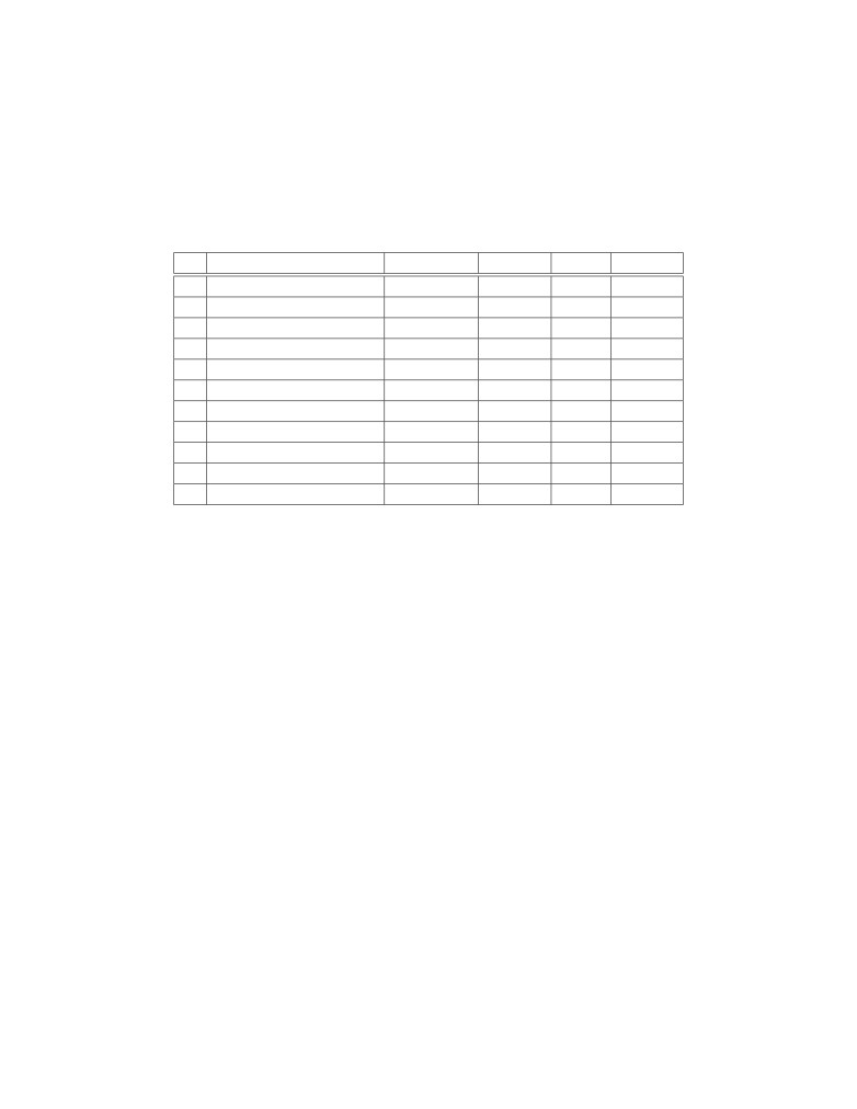
This section lists all the use cases found for the SCADA system project. This is useful
for producing tests when implementing the project program. Each use case should be easily
verifiable. These use cases were developed by naming primary actors and predicting how
they would use the SCADA system:
N
Use Case:
Researcher
Student
Guide
Priority
1
Notification system
x
1
2
Indefinite SCADA run
x
1
3
System log
x
1
4
Display Live Data
x
1
5
Transform Data
x
x
x
3
6
Calibrate Sensor
x
x
2
7
Sample Sensor
x
x
2
8
Display Data
x
x
2
9
Access Database
x
x
x
2
10
Test Sensor
x
1
11
Export Data
x
x
2
Table 1: This table shows the priority of the use cases for the SCADA system.
1.5
Additional Constraints
In addition to the information gathered from initial customer meetings, there a few
additional constraints. To keep the bulk of the project focused on the data management of
the SCADA system, Phidgets USB Sensors were selected to be the exclusive sensor. The
Phidgets company provides a C library and API for interfacing with the hardware. This
reduces the amount of low level work required for communicating across USB. Additional
advantage of the Phidgets selected for use with this project work is that they utilize a hub
system. This emulates the hub system that is found in more commonly used communication
interfaces such as CAN bus. In these systems, sensors are associated with a data acquisition
hub (DAQ). Thus information sent over the data bus will always have some hub identifier.
4
2
System Design
2.1
Component Overview
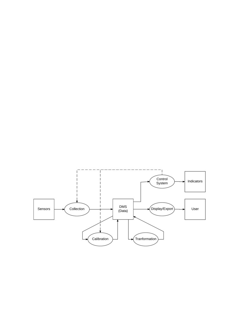
In order to accomplish the tasked listed in Section 1.4, the system will be broken into
components that will operate somewhat independently. The major design components for
the SCADA system in this report include the Data Management System, Collection System,
Calibration System, Transformation System, Control System, and a Export System. Figure
1 shows how the major design components work to accomplish the design goals discussed in
the prior sections.
The flow of data through the system starts with the sensors as they are the source of
data for the project. The Collection System will manage the sampling settings and data
acquisition for each sensor. Additionally, the Collection System will write the sampling data
to the Data Management System (DMS). Once there is data in the DMS, the Calibration
System can apply calibration models to allow for a real-world interpretation of the data.
The Calibration System will write calibrated data back to the DMS for storage and later
usage. The system is able to further manipulate data through the Transformation system
by applying averages and combining data through various mathematical operations. In
addition to storing the sample data by the SCADA system, the DMS is also responsible for
data archival.
Figure 1: Square boxes represent physical locations where data is utilized or stored. Ovals
represent system processes for the creation and manipulation of data. Solid lines show the
flow of data.
5
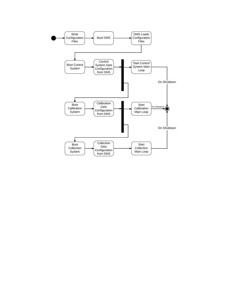
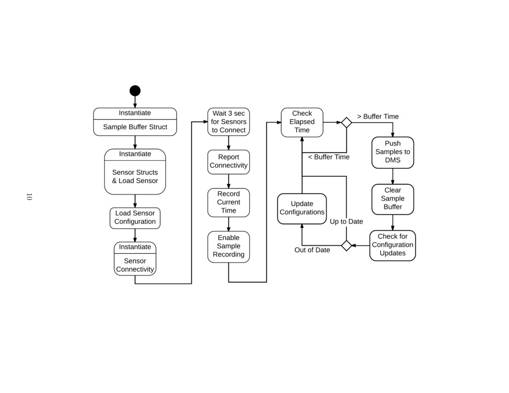
Figure 2: This diagram shows the system start up and how each independent system process
is started. The transformation system is not included in this diagram but would be started
in a similar fashion after the calibration system.
The SCADA system can react to the all three types of data through the Control System.
The user will define the conditions to perform various actions through the Control System.
Such actions can involve changing the state of indicator outputs or changing how data is
collected and manipulated. The Export System will be able to filter and export data so
that the user can perform post analysis. The export functionality will be able to output
spreadsheets as these are forms that user is able to interact with directly and use in 3rd
party data analysis tools.
2.2
Data Management System
The Data Management System (DMS) is designed to serve several purposes within the
overall SCADA system. The primary purposes of the DMS is to store data, manage the
6
configuration of other systems, and act as an interface between other systems. The DMS
manages the configurations of other systems so that the user and other systems can specify
what set of configurations to use at any given time. An example of this is the configuration
for the Collection System. It is important that Control System is able to select what the
current Collection configuration as this was a design requirement provided by the customer.
It is important that the DMS manages these configurations as it will prevent separate systems
from having access to each others configuration files directly. Thus inter-system dependency
is reduced by using the DMS as the interface.
The DMS consists of an SQ-Lite database and additional functions wrapping SQ-Lite
API. The wrapping was designed to give the user flexibility to view data as well as write
conditions for the Control subsystem. In implementation, the DMS can handle a string
formatted in SQL to configure the system. However, the DMS was designed against a full
SQL API wrap to limit the access the user had to the table architecture and to keep the
information that the tables contain non-corrupted. The SCADA system uses a database
because an SQ-Lite database can be designed to reduce redundancy and create associations
between data sets, which makes it well adapted for user post-analysis.
The DMS, when booted up, uses the configuration file found in the project repository
called “deftables.txt”. This file creates the structure of the database as seen in the table-view
figure. It then stores references to those tables in a vector so that other systems can call
wrapped C++ methods for the SQ-Lite API and either influence a given table or read from
it. The DMS also contains an object that tracks the current state. This is tracked so that
the subsystems can easily find the up-to-date state of the SCADA.
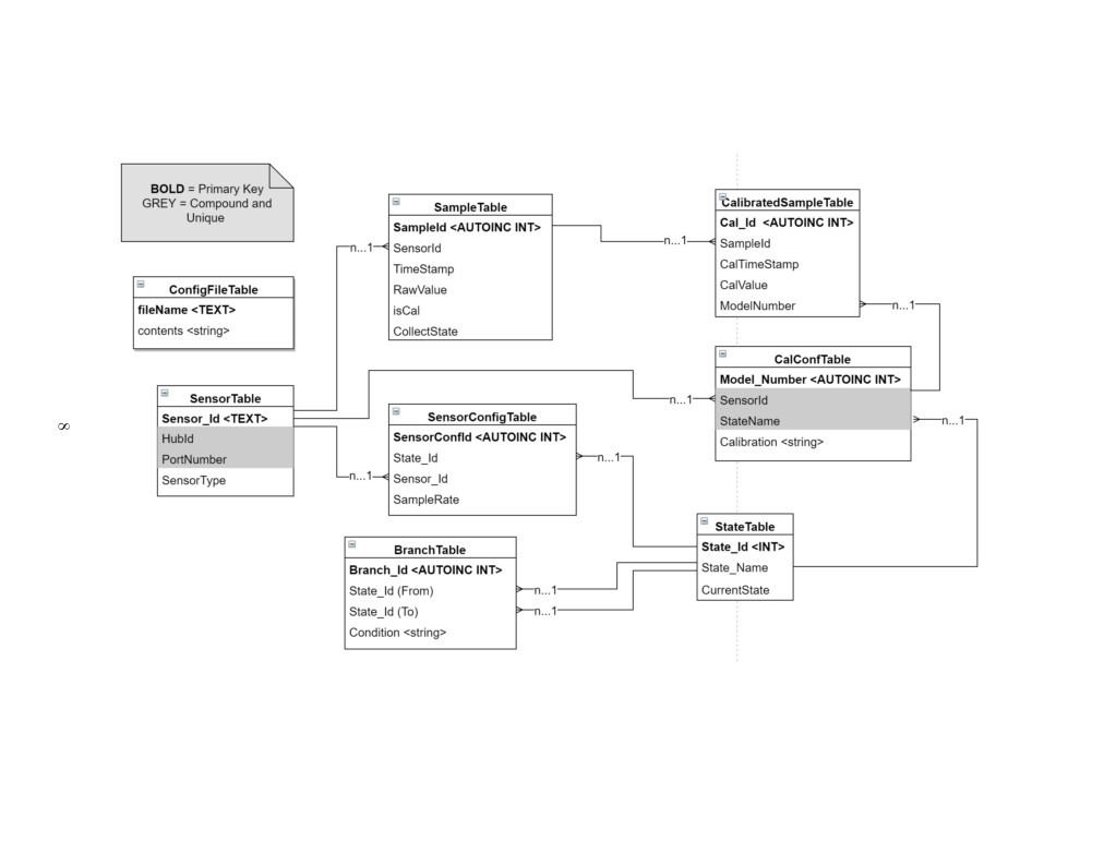
The table-view figure is a map of the table architecture for the database. Due to the
inter-connectivity of the SCADA systems information: sensor names, state names, hub ids,
and port numbers, the database is designed to define the SCADA structure before collecting
data. The tables that must be configured before this process is run are the ConfigFileTable,
the SensorTable, and the StateTable. These are defined first because the system needs to be
aware of what architecture it’s running on.
The ConfigFileTable addresses a file name to it’s contents. This is stored because the
other SCADA subsystems define their system processes from their configuration during run-
time, in the event that the user changes the configuration. The SensorTable addresses a
unique Sensor Id to a Hub Id, Port Number, and then a sensor type. This information
allows configures what the SCADA expects to see from the collection subsystem. A sensor
needs to be defined in configuration so that the SCADA is aware that it is collecting from
that sensor. The StateTable addresses all of the States that are necessary for the control
subsystem. This table details the names for states so that the control architecture can be
configured.
7
Figure 3: This diagram shows the architecture for the database.
Following these tables is the SampleTable, which is where all the raw sensor data is stored.
This information is associated with the sensor id, time-stamp, as well as an “isCal” boolean,
and a Collection State. The Sensor id, time-stamp, and Collection State allow the user to see
the context and relevance of the raw data. The “isCal” allows the system to see if the data
in a given row has been calibrated. The CalConfTable stores a user-defined calibration for a
given sensor depending on state. This table acts as an archive for the calibrations in a given
state, so that the SCADA can update each calibration during run-time. The BranchTable
defines the Control subsystem architecture by connecting defined states and the condition
that will trigger the state change.
Finally, the last Tables that are defined are the CalibratedSampleTable as well as the
SensorConfigTable. The CalibratedSampleTable stores the calibrated values of raw data,
with the time of calibration, and the sample it’s associated to. In addition, the Model-
Number is given so that the user may track what calibration is given to the sample. The
SensorConfigTable provides the sampling rate for independent sensors.
2.3
Collection System
The collection system is responsible for managing the array of sensors. This includes
scheduling when to sample sensors and managing sensors sampling parameters. The Phidget
API includes a variety of methods for managing sensors. There are two ways that sensors
can be samples: polling and events. The Phidgets company states that it is recommended
to use sampling events as it is the most robust and reliable way of sampling. Due to this
statement, the design implemented utilizes sampling events. Additionally, this allows for a
reliable and efficient way to provide individual sampling period for each sensor. Further, the
use of sampling events is fast and limits the sampling period of sensors to the time required
to handle a sampling event. This breaks the collection system into system initialization,
sample event handling, and the main loop.
On initialization, the collection system must perform the following tasks.
• Create the required data structures for holding sensor and sample data
• Open a connection to the database and load sensor information
• Check the backup sample file to ensure that no samples were missed due to system
failure
• Create connections to the Phidget Sensors and instantiate collection
9
Figure 4: The collection main process has two distinct stages: instantiation and the main loop. The backup sample file process
is not explicitly shown above.
When Phidgets are initialized, a sampling period is specified according to the information
pulled from the database. This sampling period is used to trigger sampling events the
specified time has elapsed. Until the collection system is initialized, all samples will not be
record. This is to ensure that all data is valid. Once the system is initialized, the system is
set to record samples and the process enters the main loop.
When a sensor sampling time has elapsed, a sampling event happens automatically. This
is handled by the function attached to the onVoltageChangeHandler in the PhidgetVolt-
ageInput class. When an event occurs, a time stamp is immediately recorded to ensure that
the most accurate time stamp is recorded. The time stamp is a single numeric specifying the
number of milliseconds since the 1970 epoch. Then the system uses the attached reference
to the Sensor struct to obtain additional information about the sensor needed to prepare the
sample entry string. Such information includes the sensorName. Through the sample struct,
the event handler also checks that the system is recording samples. This is done to ensure
that the collection system had ample time to start up. While not currently implemented,
the ability to disable collection would allow a human user or the control system to disable all
sensor recording if desired. If the system is recording samples, the a sample string is created
containing all the information required by the DMS to record a sample. All new samples
have a default “isCal” value of 0 as new samples will not have been calibrated when entered
into the database. Once the string is constructed it is added to the sampleBuffer which is
implemented as an array of character pointers. Additionally, the string is appended to the
“sampleBackup.txt” file.
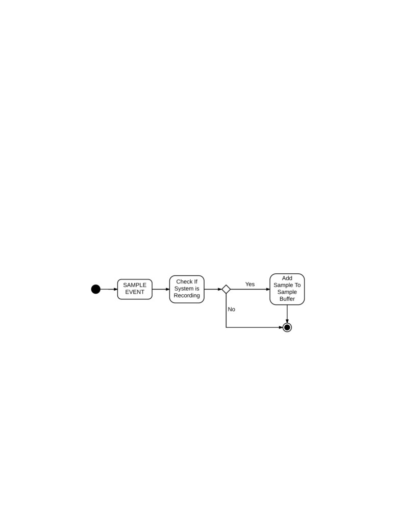
Figure 5: Sample events create a time stamp when creating. Each event must check whether
the system is recording samples to ensure the system has instantiated.
The main loop of the collection process has two functions. The first is to manage pushing
all of the samples in the sample buffer to the database. A sample buffer is required to prevent
the collection system from over accessing the database and locking the database, preventing
other systems from accessing the database. This is done by checking the amount of elapsed
time from the last time the system pushed the samples to the database. When the time has
elapsed, all samples are entered into the SampleTable of the database. Once this is done,
the sample buffer and the sample file backup are cleared. Additional, the main loop must
check the database to see if the current state has changed. This is done every time the
system pushed samples to the database. If the current state has changed the new sensor
11
configurations are retrieved from the database and the running sensors are updated in a
process similar to Phidget initialization.
*Note about Phidget22 C Library: As of November 29th, 2017, it was found and firmly
established that the Phidgets22 C Library is incompatible with the GNU C++ compiler.
This was confirmed verbally with other groups that were also unable to directly incorporate
Phidgets22 Library code within additional C++ code. This caused a delay in the develop-
ment of the control system because it required changing the design of the control system
to its current form (presented above). Additionally, it was unable to use the DMS wrapper
object as it was written in C++. Thus the collection system had to interface directly with
the SQLite database.
2.4
Calibration System
The Calibration subsystem is a pivotal part of the SCADA. This system allows for the
raw data from sensors to have real analytic meaning. When the user is looking to collect
meaningful data from several sensors that aren’t identical, it becomes important to calibrate
accordingly to make a uniform model for the behavior of any collected data.
The Calibration subsystem interacts with the raw data that is stored in the DMS from
the Collection subsystem. The Calibration subsystem will check for data and calibrate it
to the calibration that was associated with the collecting sensor. This calibration is user
defined in the configuration and can be changed to allow for more accurate calibration.
After calibration, these new data points would then be stored back into the DMS according
to the sample id, the time of calibration, and the calibration model that is associated to the
sample.
2.5
Transformation System
The Transformation System is used to apply further mathematical operations to the data.
The transformation system will operate similarly to the calibration system in that it will pull
new data that has not yet been transformed from the SampleTable in the DMS. Thus every
transform will for a primary sensor source used for sample indexing. The transformation
system will support a a variety of operations and allow for the additional functionality to
be implemented. There are two main types of transformation that the system will support:
single source averaging and multiple source arithmetic operations.
Single source averaging involves taking data from previously collected cycles and using
an averaging technique on those collected points. The user first needs to provide a sensor
source for averaging use. Then the user can specify the type of averaging use. The user will
be able to select between mean, median, and mode as averaging types. Additionally, the
12
user can select the averaging window size. This value can be given in number of samples or
time period. Finally, the user should be able what time stamp is recorded for the specific
averaging windows. Usually this is the average time of the window. However, the user will
also be able to select the first and last time as time stamp options for the averaged sample
point.
The multiple source transformation type is defined in a generic way such that its func-
tionality can be expanded as more arithmetic operations are added by the developer. A basic
set of operations will include addition multiplication with sensor samples and constants. An
example of such an operation is taking calibrated data from a voltmeter and an ammeter
and multiplying them to create a power data point. One complication of the abstract of the
configuration system is that sensor are not guaranteed to sample at the same time and at
the same frequency. This can be corrected in a few ways.
One way to fix this indexing issue can be found by first simplifying the issue. Assume
that the sensors being transformed are sampled at the same frequency but have some phase
offset. There is a natural one-to-one correspondence between the samples of the two sensors.
If the one-to-one correspondence is loosened, the correspondence naturally becomes samples
that are closest in time. This is a strong relationship to use for sample correspondence within
the transformation system as it can be implemented fairly easily and it can be applied to
signals that do not have the same sampling frequency. This is the approach that will be
initially implemented for the transformation system.
2.6
Control System
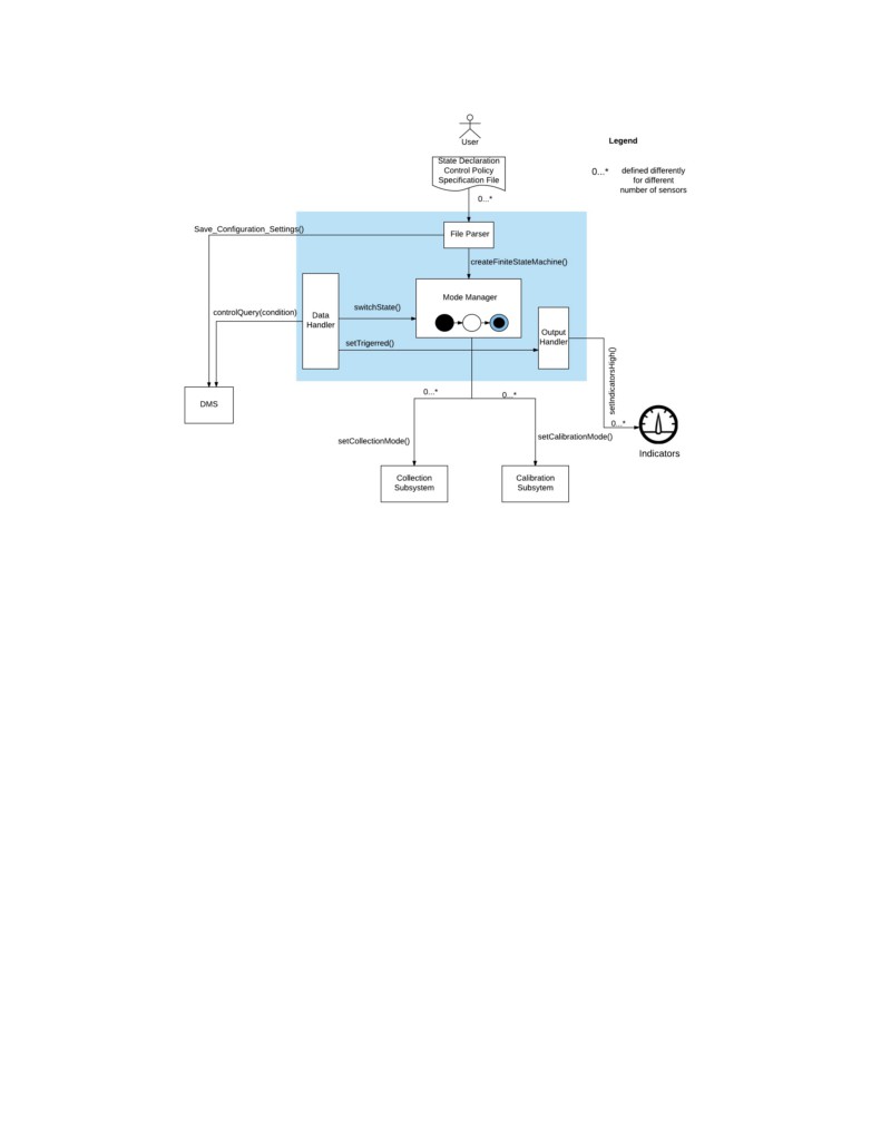
The Control System, as shown in Figure 6 contains four major components, and they are
described in the following subsections.
2.6.1
File Parser
This component reads in a configuration file given by the user. The configuration file
includes configurations for the mode manager, the sensor architecture, the collection, and the
calibration collection systems. The file parser fills the information in the respective tables of
the DMS by saving all the configuration settings. This is invaluable to the system because
each system can easily access any information from the DMS. The configuration file and its
format including the syntax is described later in section 3.2.
13
Figure 6: Control Subsystem Overview
2.6.2
Mode Manager
The Mode manager looks for its configuration setting in the DMS and creates a finite
state machine that indicates modes of collection and modes of calibration. One instance
where the mode manager could be important is when a user decides to collect and calibrate
data differently. The mode manager declares states, defines the branch/transition conditions,
and most importantly indicates the current state in the DMS so that the collection and the
calibration systems respectively pick the appropriate mode that corresponds to the current
state. The mode manager also performs branches to next state with the switchState()
instruction which is executed when a branch condition is found to be true. As described
above whenever a state branch has been taken, the mode manager updates the current state
variable in the DMS.
2.6.3
Data Handler
The data handler, based on the state the mode manager is in, checks if any of its branches
can be taken by running a query of the condition in the DMS. If any of the branches can
be taken, it instructs the mode manager to switch to the respective state. In addition, the
data handler checks if a trigger value has been reached and sends the setTriggered() signal
14
to the output handler that sets indicators on and off as well as indicate the current state.
2.6.4
Output Handler
The output handler essentially looks at the setTriggered() signal from the data handler
and turn indicators on and off as needed. This also includes indicating the current state of
the system.
2.7
Data Export System
The export system was designed to simply query the database for the information ac-
cording to the user input and then generate a file containing the according information.
This feature is implemented through the DMS. In order to export, all that is necessary is a
specified query from the user, assuming that they know SQLite query formatting, they can
input this directly into the DMS. The Export makes it easier for the user to take the data
from the SQLite database and use it in other application, such as Matlab or Excel.
2.8
Configuration Utility
The Configuration Utility is the tool which allows the user to setup up the SCADA
system. This was designed to display the actual configuration file to the user and allow them
to edit it. The edits would then be stored into the system and run under a configuration
error handle. However, in implementation we were only able to create a error handler that
caught errors in the state and branch conditions. The content of these files are then stored
into the database so that the other systems can access and configure their own parameters
accordingly.
The Graphical User Interface (GUI) was specified by the user to be less significant overall
to the system performance. Less focus went into this design than into others. This was
designed, instead of a main component, as just a utility for configuring the SCADA system
as well as visualizing and exporting data. The GUI has the capability of showing current
configurations of the SCADA system. This design is a good fit into the overall SCADA
system because it is functional, which is a user story as defined earlier.
The GUI is shown in the following figures:
15
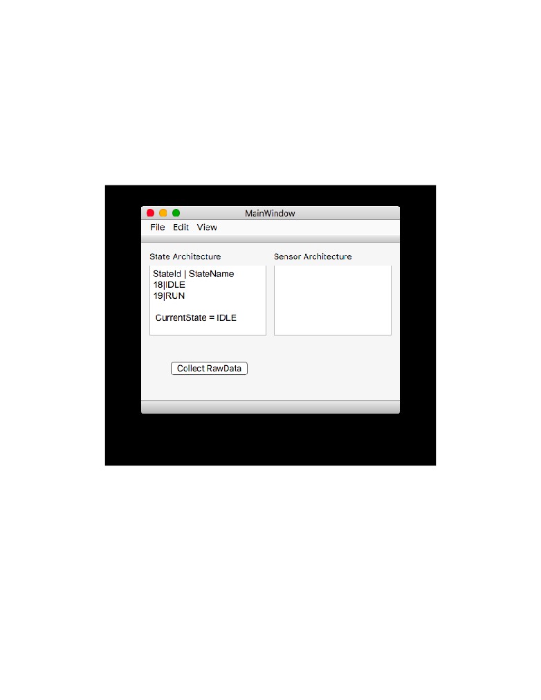
Figure 7: The Main Window for the GUI shows the current configuration of the states and
sensors in the SCADA according to the current configuration file. The window also allows
the user to configure, export, or view the current database from the menu bar.
16
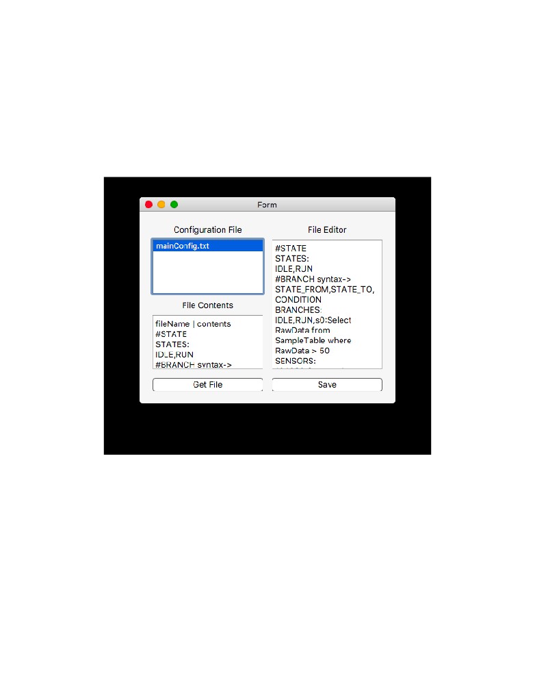
Figure 8: The Configuration Window shows the configuration files that are listed. Once
selected the preview window will show the contents of the file before allowing the user to
edit it. Once the user selected a file, it’s contents are displayed on the right window. In this
window the user can edit the file and save their changes.
17
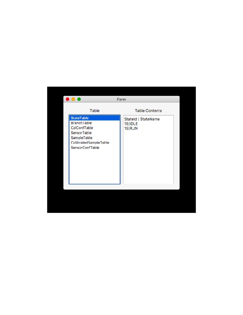
Figure 9: The TableView Window shows the contents within the database, according to the
selected table.
18
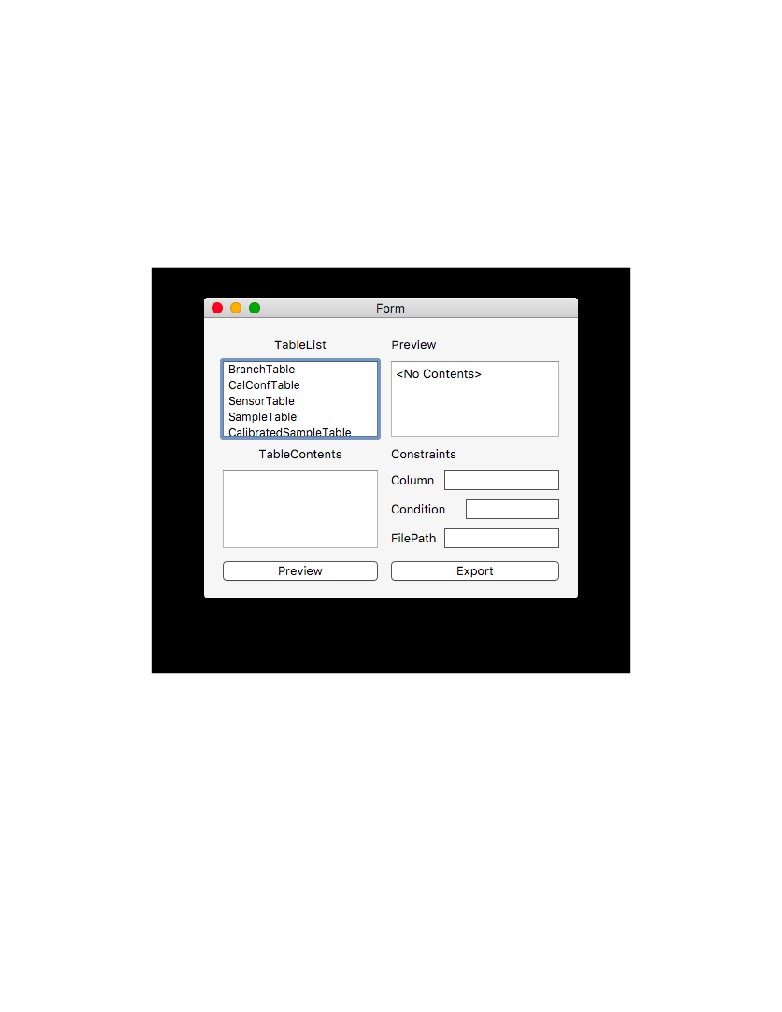
Figure 10: The Export Window allows the user to specify the a table, and then the constraints
in the line edit widgets to specify the data being exported. Once exported a file window will
appear for the user to specify the location of the export file.
19
3
User Manual
Upon boot the user will be able to see the GUI. This GUI will open the database and allow
the user to analyze the information contained in the database. However, due to development
issues, the collection system was difficult to integrate with the rest of the system. The main.c
file must be compiled in the terminal window and the executed. This will then start adding
data to the database from the Phidget devices.
3.1
Configuration
Configurability was a major part of our design. It was central to the idea of the customers
dream system. Due to this, we tried to format a way to configure the entire system before
running it. The setup utility (used in the GUI) allows the user to do exactly that. The user
can declare collection modes, store calibrations, sensor architectures, control states, as well
as branch conditions. The configuration file was formatted to take user configuration in one
file, so that the user had to correct the errors all at once.
User declares states with the header “STATES:” and in the following line lists the state
names separated by a comma. The system requires the first state in the list to be a default
current state. In addition, it requires the names of the state to be dissimilar.
User defines branches by defining the state the branch is starting from, the state where it
is heading to, and the condition for the branch to be taken. The system checks if the states
are declared in the state declaration. If not, it prompts the user the error. The condition
takes in a SQL query, and the system checks in if the query holds true and decides if the
branch can be taken. The branch configuration was formatted under the assumption that
the user knew SQL.
User declares sensor architecture with the HubId, the port number and the name of
the sensor. In addition, the user can also declare calibration with a sensor name, listed
in the declaration of sensor architecture, a state associated with the calibration, and the
calibration mode. The system supports linear and quadratic calibrations. The collection
system is defined similarly. The user adds in “END” at the end of the configuration file to
signal an end to the document. The user can use “#” for commenting purposes.
STATES :
<StateName0><StateName1 > . . .
BRANCHES:
<FROMSTATE>,<TOSTATE>,<CONDITION>
SENSORS :
<HUBID><PORTNUMBER><SENSORNAME>
20
CALIBRATION :
<SENSOR><STATE><CALIBRATION>
COLLECTION :
<SENSOR><STATE><SAMPLINGRATE>
END
(Comments are Preceded by a #)
( Conditions are written in SQL Format)
Ex .
#STATE syntax−> <STATE 1 Name>,<STATE 2 Name>,<STATE 3 Name>
STATES :
IDLE ,RUN, STOP
#BRANCH syntax−> <STATE FROM>,<STATE TO>,<CONDITION>
#where <CONDITION> i s <SENSOR ID : SQL QUERY>
BRANCHES:
IDLE ,RUN, s 0 : S e l e c t RawData from SampleTable where RawData >
2.0
RUN, STOP, s 1 : S e l e c t RawData from SampleTable where RawData > 2 . 5
STOP, IDLE , s 1 : S e l e c t RawData from SampleTable where RawData <
2.5
#SENSORS syntax−> <HUB ID>,<PORT NO>,<SENSOR ID>
SENSORS :
4971941,1,s0
4953315,5,s1
#CALIBRATION syntax−> <SENSOR ID>,<STATE NAME>,<CALIBRATION>
#where <CALIBRATION> i s <t y p e : c o e f f s l i s t e d with
:>
CALIBRATION :
s0 ,IDLE, linear :2:1
s1 ,IDLE, linear :2:1
s0 ,RUN, linear :2:1
s1 ,RUN, linear :2:1
s0 ,STOP, quad :2:3:1
#COLLECTION syntax−> <SENSOR ID>,<STATE NAME>,<SAMPLING PERIOD>
COLLECTION :
s0 ,IDLE,2000
s1 ,IDLE,2000
s0 ,RUN,750
s1 ,RUN,750
s0 ,STOP,750
END
21
4
Implementation Results & Future Work
The collection system was not fully implemented due to timing constraints and difficulty
of learning to work with C and the Phidgets API. All major interfaces have been implemented
and tested. This includes reading and storing sensor informaton from the database, writing
samples to the database, and collecting samples from sensors. The event based sample
collection system performed extremely well in an informal stress test. The system was able
to handle four sensors being at different rates under 700 milllisecond. This exceeded the
customers specification of a minimum sampling rate of 1 second. It would likely require
on couple weeks to implement the remaining functionality of the collection system. This is
includes:
• Correctly storing the current state from the database
• Updating the sensor configuration at the end of pushing the sample buffer
• Reading the SampleBackup file at start and pushing any samples to the database.
Due to the reliability and performance of the collection systems basic features, the collection
system is at its core very developed despite lacking features.
The GUI could be designed to be more aesthetically appealing, as well as more powerful.
Because of time-constraints, we were not able to cover the error-handling in the GUI, this
allows the user to make mistakes and cause problems in the system, which is non-ideal. It
would also be a future design consideration to the Transformation system. Considering that
our group size was one of the smallest we did not have enough time nor work power to finish
all of the capabilities of the SCADA system specified in the user stories. However, in the
future this will be part of the design.
5
References & Resources
Design Process
• Miles, R., and K. Hamilton. Learning UML 2.0. OReilly, 2006.
• “A Quick-Start Tutorial on Relational Database Design.” Relational Database
Graphical Documentation
• Lucid chart
• draw.io
22
Collaborative Documentation
• Git repository
• Google Drive
• ShareLatex
Coding Implementation
23